Compare Power from RMSTdesign and SSRMST Packages
Source:vignettes/Compare-to-SSRMST.Rmd
Compare-to-SSRMST.RmdThis vignette compares results from our package and the SSRMST package. The data is based on the Saxagliptin Study which studied the cardiovascular risk of saxagliptin.1,2 We compare results from the SSRMST package with the RMSTdesign package. The SSRMST package calculates power based on simulations for trials with Weibull distributed survival times.
The accrual rate, accrual period, trial time, Weibull shape and scale parameters of the control (arm0) and treatment (arm 1) distributions, and tau were set according to the example. The results from the ssrmst function are shown below.
ac_rate   = 30
ac_period = 70
tot_time  = 908
shape0 = 1.05
shape1 = 1.05
scale0 = 8573
scale1 = 8573
tau  = 900
ssrmst(ac_rate=ac_rate, ac_period=ac_period, tot_time=tot_time, tau=tau, shape0=shape0, scale0=scale0, shape1=shape1, scale1=scale1, seed=2017)
#> Superiority test
#>
#>                           Total arm0 arm1
#> Sample size                2100 1050 1050
#> Expected number of events   182   91   91
#>
#> Power (separate)
#>            0.028
#> Power (pooled)
#>          0.028
Using RMSTdesign, the following code calculates the power under the same trial design assumptions.
arm0<-survdefWeibull(shape = shape0, scale = scale0)
arm1<-survdefWeibull(shape = shape1, scale = scale1)

RMSTpow(arm0, arm1, k1=70, k2=908-70, tau = 900, n=30*70)
#> $n
#> [1] 2100
#>
#> $powerRMST
#> [1] 0.025
#>
#> $powerRMSTToverC
#> [1] 0.025
#>
#> $powerRMSTCoverT
#> [1] NA
#>
#> $powerLRToverC
#> [1] 0.025
#>
#> $powerLRCoverT
#> [1] NA
#>
#> $powerLRtauToverC
#> [1] 0.025
#>
#> $powerLRtauCoverT
#> [1] NA
#>
#> $pKME
#> [1] 1
In the output of the RMSTpow function, we should focus on the quantity powerRMSTToverC, which is the asymptotic power of the restricted mean-based test for the superiority of treatment over control. The output of the ssrmst function gives the empirical power of the same test based on simulations (2000 simulations by default). We see that we get similar results with the two packages, and that, as expected under the null scenario, the null hypothesis is rejected about 2.5% of the time, which is equal to the one-sided alpha level.
Next, consider a scenario where the alternative hypothesis is true and compare the power obtained using the two packages.
arm1alt<-survdefWeibull(shape = shape1, scale = 16000)
plotsurvdef(arm0, arm1alt, xupper = 1000)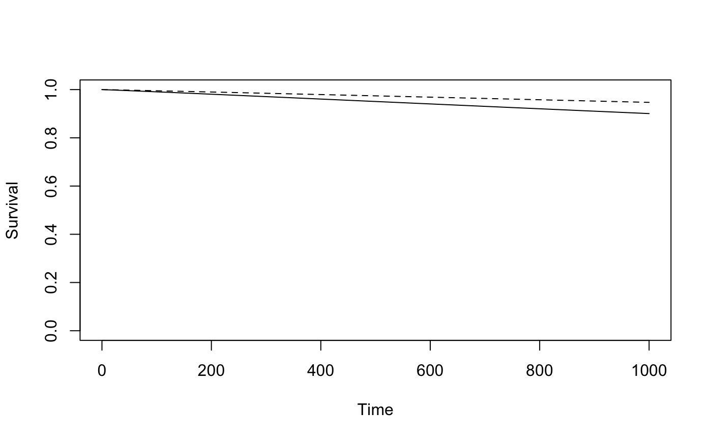
ssrmst(ac_rate=ac_rate, ac_period=ac_period, tot_time=tot_time, tau=tau, shape0=shape0, scale0=scale0, shape1=shape1, scale1=16000, seed=2017)
#> Superiority test
#>
#>                           Total arm0 arm1
#> Sample size                2100 1050 1050
#> Expected number of events   139   91   48
#>
#> Power (separate)
#>            0.917
#> Power (pooled)
#>          0.917

RMSTpow(arm0, arm1alt, k1=70, k2=908-70, tau = 900, n=30*70)
#> $n
#> [1] 2100
#>
#> $powerRMST
#> [1] 0.9113981
#>
#> $powerRMSTToverC
#> [1] 0.9113981
#>
#> $powerRMSTCoverT
#> [1] NA
#>
#> $powerLRToverC
#> [1] 0.9632719
#>
#> $powerLRCoverT
#> [1] NA
#>
#> $powerLRtauToverC
#> [1] 0.9631907
#>
#> $powerLRtauCoverT
#> [1] NA
#>
#> $pKME
#> [1] 1
Again the power returned by both packages is similar: 91.7% for the SSRMST package, and 91.1% for the RMSTpow package.
Next, consider changing tau to 450.
ssrmst(ac_rate=ac_rate, ac_period=ac_period, tot_time=tot_time, tau=450, shape0=shape0, scale0=scale0, shape1=shape1, scale1=16000, seed=2017)
#> Superiority test
#>
#>                           Total arm0 arm1
#> Sample size                2100 1050 1050
#> Expected number of events   139   91   48
#>
#> Power (separate)
#>            0.637
#> Power (pooled)
#>          0.637

RMSTpow(arm0, arm1alt, k1=70, k2=908-70, tau = 450, n=30*70)
#> $n
#> [1] 2100
#>
#> $powerRMST
#> [1] 0.6368899
#>
#> $powerRMSTToverC
#> [1] 0.6368899
#>
#> $powerRMSTCoverT
#> [1] NA
#>
#> $powerLRToverC
#> [1] 0.9632719
#>
#> $powerLRCoverT
#> [1] NA
#>
#> $powerLRtauToverC
#> [1] 0.7607574
#>
#> $powerLRtauCoverT
#> [1] NA
#>
#> $pKME
#> [1] 1
Again, the power returned by both packages is similar: 63.7% for the SSRMST package, and 63.7% for the RMSTpow package.
Finally, consider changing the accrual period to 35 months.
ssrmst(ac_rate=ac_rate, ac_period=35, tot_time=tot_time, tau=tau, shape0=shape0, scale0=scale0, shape1=shape1, scale1=16000, seed=2017)
#> Superiority test
#>
#>                           Total arm0 arm1
#> Sample size                1050  525  525
#> Expected number of events    71   46   25
#>
#> Power (separate)
#>            0.655
#> Power (pooled)
#>         0.6535

RMSTpow(arm0, arm1alt, k1=35, k2=908-35, tau = 900, n=30*35)
#> $n
#> [1] 1050
#>
#> $powerRMST
#> [1] 0.6481269
#>
#> $powerRMSTToverC
#> [1] 0.6481269
#>
#> $powerRMSTCoverT
#> [1] NA
#>
#> $powerLRToverC
#> [1] 0.7637835
#>
#> $powerLRCoverT
#> [1] NA
#>
#> $powerLRtauToverC
#> [1] 0.763348
#>
#> $powerLRtauCoverT
#> [1] NA
#>
#> $pKME
#> [1] 1
Again, the power returned by both packages is similar: 65.5% for the SSRMST package, and 64.8% for the RMSTpow package.
Scirica BM, Bhatt DL, et al. Saxagliptin and Cardiovascular Outcomes in Patients with Type 2 Diabetes Mellitus. N Engl J Med. 2013, 369, 1317-26.↩
https://cran.r-project.org/web/packages/SSRMST/vignettes/vignette-ssrmst.html↩