Using RMSTdesign to Find Optimal Trial Designs • RMSTdesign

library(RMSTdesign)

We use a simple example to discuss different criteria for selecting an optimal trial and how to do it. In some cases the optimal trial design may be the one that has the smallest sample size, regardless of duration; in other cases it may be the one with the shortest duration, regardless of sample size, and in other cases, you may be looking for a balance between the two.

We consider planning a trial where we expect survival time distributions in both the control and treatment groups follow exponential distributions, which implies proportional hazards. We expect the median survival time in the control group to be 3 years and the new treatment to reduce mortality risk by 33% (hazard ratio = 0.67). In the disease we are studying, 3 years is a clinically important landmark, so we choose \(\tau\)= 3 years. We plan to do a one-sided test, and we want to estimate the sample size to achieve 80% power with a one-sided Type I error of 0.025.

con<-survdef(times = 3, surv = 0.5) 
trt<-survdef(haz = 0.67*con$h(1))
plotsurvdef(con, trt, 5)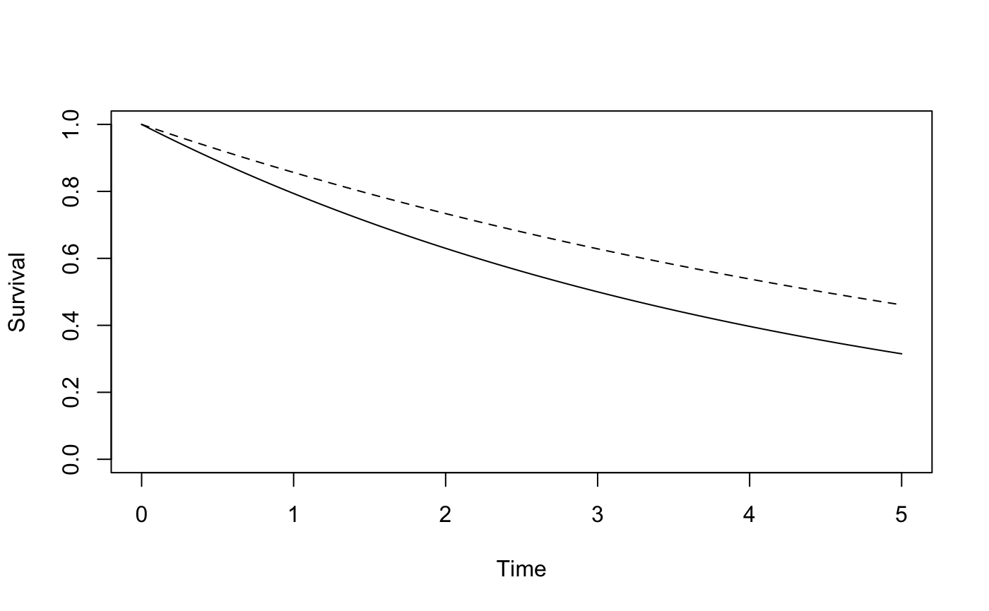

We can consult Table 2 to get a rough estimate of the number of patients we will need for a hazard ratio of 0.67 with \(\tau\) equal to median survival in the control group. We will need 552 patients (276 in each arm) to achieve 80% power. This estimate doesn’t take into account administrative censoring. This code obtains the same result.

RMSTpow(con, trt, k1 = 0, k2 = 3, tau = 3, power = 0.8)
#> $n
#> [1] 552
#> 
#> $powerRMST
#> [1] 0.8008182
#> 
#> $powerRMSTToverC
#> [1] 0.8008182
#> 
#> $powerRMSTCoverT
#> [1] NA
#> 
#> $powerLRToverC
#> [1] 0.8708721
#> 
#> $powerLRCoverT
#> [1] NA
#> 
#> $powerLRtauToverC
#> [1] 0.8708721
#> 
#> $powerLRtauCoverT
#> [1] NA
#> 
#> $pKME
#> [1] 1

The trial with all patients followed to time \(\tau\) is optimal in terms of minimal sample size. Also, you are sure to be able to estimate RMST difference at time \(\tau\) because no patients will be censored before time \(\tau\). Note that extending followup time beyong \(\tau\) provides no benefit in terms of either power or pKME (the probability RMST difference will be estimable with the Kaplan-Meier estimator), though it does increase the power of the standard log-rank test calculated with all avaiable follow-up (the quantity powerLRToverC in the output below).

RMSTpow(con, trt, k1 = 0, k2 = 10, tau = 3, power = 0.8)
#> $n
#> [1] 552
#> 
#> $powerRMST
#> [1] 0.8008182
#> 
#> $powerRMSTToverC
#> [1] 0.8008182
#> 
#> $powerRMSTCoverT
#> [1] NA
#> 
#> $powerLRToverC
#> [1] 0.9908296
#> 
#> $powerLRCoverT
#> [1] NA
#> 
#> $powerLRtauToverC
#> [1] 0.8709119
#> 
#> $powerLRtauCoverT
#> [1] NA
#> 
#> $pKME
#> [1] 1

We may also be interested in the trial design with the shortest duration. Our function shortest_duration can find that design, but you need to input an accrual rate. Let’s assume the accrual rate is 552/4 = 138 patients per year. Notice that under this assumption, accruing 552 patients takes 4 years, and a trial where you accrue 552 patients and follow all patients for 3 years takes 7 years to complete.

This code finds the shortest duration trial that has the specified power and pKME (default is 0.95):

shortest_duration(con, trt, 3, .8, 552/4)
#> $n
#> [1] 668
#> 
#> $k1
#> [1] 4.84058
#> 
#> $k2
#> [1] 0
#> 
#> $duration
#> [1] 4.84058
#> 
#> $powerRMSTToverC
#> [1] 0.8006054
#> 
#> $powerLRToverC
#> [1] 0.8586702
#> 
#> $powerLRtauToverC
#> [1] 0.8219996
#> 
#> $pMKE
#> [1] 1

The shortest duration trial enrolls 668 patients and takes 4.84 years to complete.

Our shortest duration function also optimizes over sample size, within trial designs that have the shortest duration. For example, if we thought we could accrue 1000 patients per year, either a trial that recruits for the whole duration and lasts 3.013386 years, or a trial that recruits for 0.554 years, then follows patients for 2.459386 years for a total trial duration of 0.554 + 2.459386 = 3.013386 years will meet the required threshold for power and pKME, as shown below. However, the second trial needs about 1/6 as many patients (554 versus 3012). Our shortest_duration function will return the latter trial design, the smallest sample size trial out of the trials with the shortest duration.

RMSTpow(con, trt, 3.013386, 0, 3, 3.013386*1000)
#> $n
#> [1] 3012
#> 
#> $powerRMST
#> [1] 0.9996733
#> 
#> $powerRMSTToverC
#> [1] 0.9996733
#> 
#> $powerRMSTCoverT
#> [1] NA
#> 
#> $powerLRToverC
#> [1] 0.9996469
#> 
#> $powerLRCoverT
#> [1] NA
#> 
#> $powerLRtauToverC
#> [1] 0.9996469
#> 
#> $powerLRtauCoverT
#> [1] NA
#> 
#> $pKME
#> [1] 0.9500287
RMSTpow(con, trt, 0.554, 2.459386, 3, 0.554*1000)
#> $n
#> [1] 554
#> 
#> $powerRMST
#> [1] 0.8011577
#> 
#> $powerRMSTToverC
#> [1] 0.8011577
#> 
#> $powerRMSTCoverT
#> [1] NA
#> 
#> $powerLRToverC
#> [1] 0.848365
#> 
#> $powerLRCoverT
#> [1] NA
#> 
#> $powerLRtauToverC
#> [1] 0.8483505
#> 
#> $powerLRtauCoverT
#> [1] NA
#> 
#> $pKME
#> [1] 0.9517473
shortest_duration(con, trt, 3, .8, 1000)
#> $n
#> [1] 554
#> 
#> $k1
#> [1] 0.554
#> 
#> $k2
#> [1] 2.459386
#> 
#> $duration
#> [1] 3.013386
#> 
#> $powerRMSTToverC
#> [1] 0.8011577
#> 
#> $powerLRToverC
#> [1] 0.848365
#> 
#> $powerLRtauToverC
#> [1] 0.8483505
#> 
#> $pMKE
#> [1] 0.9517498

Sometimes a trial that is only a little longer than the shortest duration trial can offer a large reduction in sample size. One way to explore this is using our shortest_duration function with the option altdesign = T. You add a multiplier which defines the trial length you are willing to consider, relative to the shortest duration trial, on a multiplicative scale. For example, if you set multiplier = 1.1, the function will find the smallest sample size trial with duration equal to 1.1 times the shorest possible duration. In other words, you are willing to consider a trial that is 10% longer than the optimal trial. In the example above, the shortest possible trial was 4.84 years, so a multiplier of 1.1 indicates considering trials of length 5.3.

shortest_duration(con, trt, 3, .8, 552/4, altdesign = T, multiplier = 1.1)
#> $n
#> [1] 568
#> 
#> $k1
#> [1] 4.115942
#> 
#> $k2
#> [1] 1.202079
#> 
#> $duration
#> [1] 5.318021
#> 
#> $powerRMSTToverC
#> [1] 0.800984
#> 
#> $powerLRToverC
#> [1] 0.8894142
#> 
#> $powerLRtauToverC
#> [1] 0.8410203
#> 
#> $pMKE
#> [1] 1

We see that by extending the trial by about half a year, we can reduce the number of required patients by 100.

We now have several candidate trial designs. We can explore each design further by plotting power as a function of each design parameter using the plot = T option. We focus on the trial that enrolls 552 patients over 4 years, then follows them for 3 years. In the following plots, the red lines represent the power of the log-rank test using all available followup, the blue lines represent the log-rank test using data to time tau, and the black lines represent the power of the test for difference in RMST restricted to time tau.

RMSTpow(con, trt, k1 = 4, k2 = 3, tau = 3, n = 552, plot = T)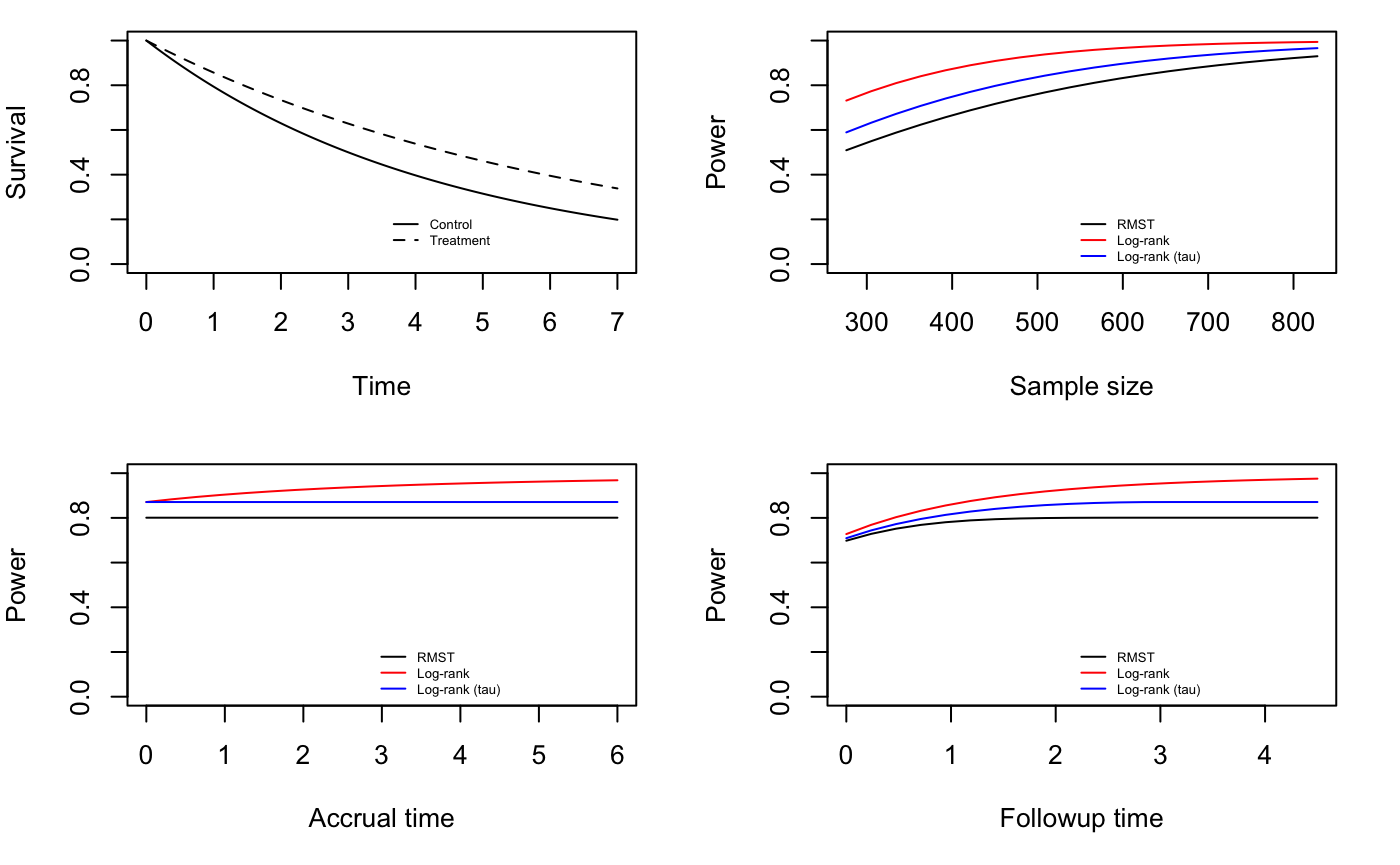

#> $n
#> [1] 552
#> 
#> $powerRMST
#> [1] 0.8008182
#> 
#> $powerRMSTToverC
#> [1] 0.8008182
#> 
#> $powerRMSTCoverT
#> [1] NA
#> 
#> $powerLRToverC
#> [1] 0.9539556
#> 
#> $powerLRCoverT
#> [1] NA
#> 
#> $powerLRtauToverC
#> [1] 0.8709213
#> 
#> $powerLRtauCoverT
#> [1] NA
#> 
#> $pKME
#> [1] 1

The plots show us that we can reduce accrual time and maintain power, but that would mean we need to enroll the same number of patients in a shorter time, which may not be practical. We also see that we could reduce follow-up time by about a year without a significant loss in power.

RMSTpow(con, trt, k1 = 4, k2 = 2, tau = 3, n = 552)
#> $n
#> [1] 552
#> 
#> $powerRMST
#> [1] 0.7998204
#> 
#> $powerRMSTToverC
#> [1] 0.7998204
#> 
#> $powerRMSTCoverT
#> [1] NA
#> 
#> $powerLRToverC
#> [1] 0.9229113
#> 
#> $powerLRCoverT
#> [1] NA
#> 
#> $powerLRtauToverC
#> [1] 0.8597414
#> 
#> $powerLRtauCoverT
#> [1] NA
#> 
#> $pKME
#> [1] 1

We see that reducing \(k_2\) to 2 went slightly too far, as power has dropped below 0.8. Using trial and error we find that \(k_2\)=2.1 is adequate to preserves power and pKME, reducing total trial duration to 6.1 years.

RMSTpow(con, trt, k1 = 4, k2 = 2.1, tau = 3, n = 552, plot = T)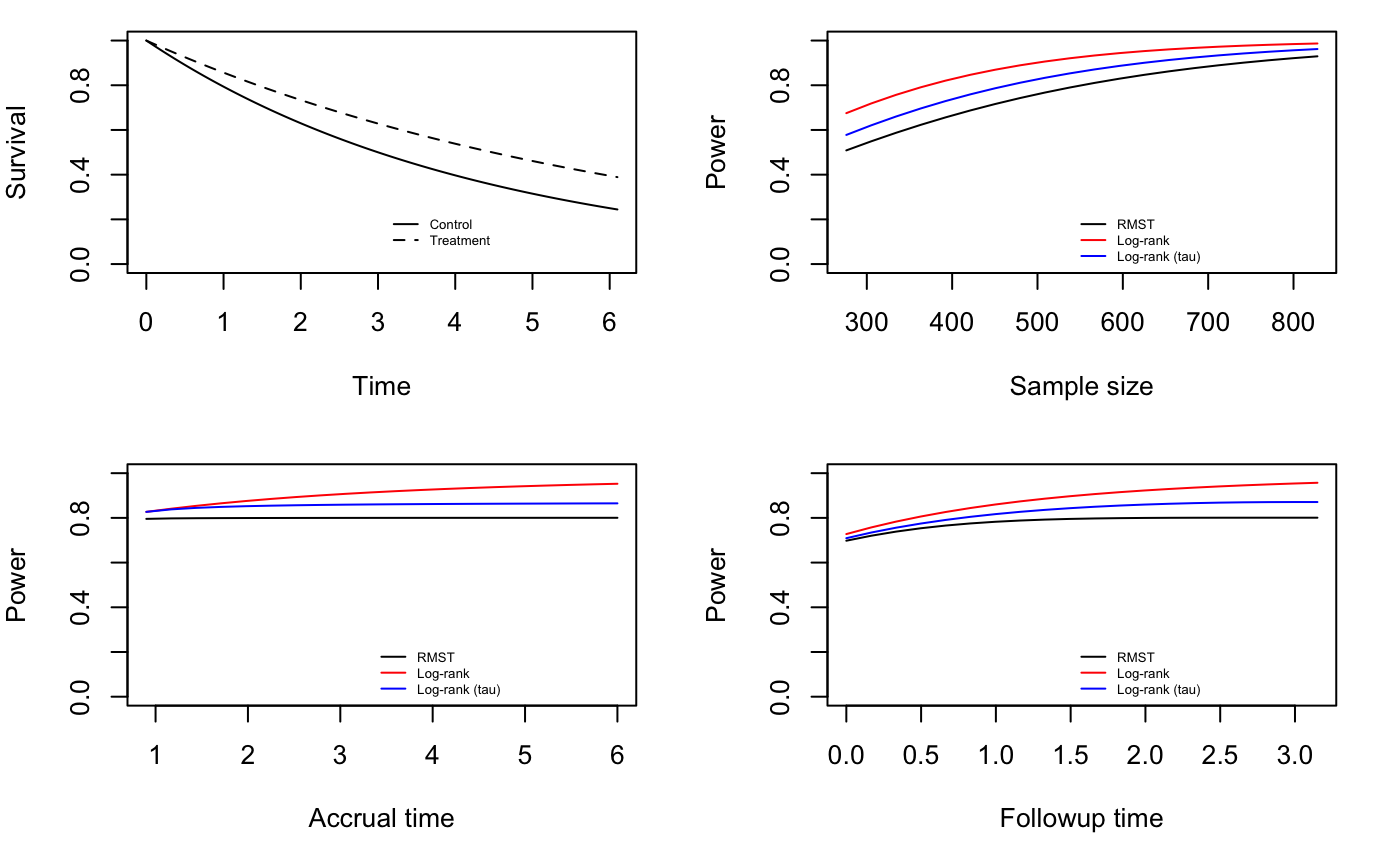

#> $n
#> [1] 552
#> 
#> $powerRMST
#> [1] 0.8001678
#> 
#> $powerRMSTToverC
#> [1] 0.8001678
#> 
#> $powerRMSTCoverT
#> [1] NA
#> 
#> $powerLRToverC
#> [1] 0.9270544
#> 
#> $powerLRCoverT
#> [1] NA
#> 
#> $powerLRtauToverC
#> [1] 0.8619928
#> 
#> $powerLRtauCoverT
#> [1] NA
#> 
#> $pKME
#> [1] 1

The plots show us that, under the new design, reducing follow-up time will reduce power. Increasing sample size or shortening accrual while keeping sample size constant would increase power, but may not be desirable or possible. Similar plots could be used to explore and tweak the other candidate designs.